Abstract
We revisit extending the Kolmogorov–Smirnov distance between probability distributions to the multi-dimensional setting, and argue for the proper way to approach this generalization. Our formulation maximizes the difference over dominating orthogonal rectangular ranges (d-sided rectangles in ℝd), and is an integral probability metric. We prove the distance between a distribution and a sample of it converges to 0 as the sample grows, and bound this rate. Up to this same error, the distance can be computed efficiently in four or fewer dimensions — near-linear in the sample size needed for that error — and we derive a δ-precision two-sample test. Finally, we show these metric and approximation properties fail for other popular variants.
Why dKS?
A distance that doesn't change when you change units
Comparing two multi-dimensional distributions comes up everywhere — deciding whether a fresh batch of data has drifted, whether two populations differ, whether a model's outputs match reality. The trouble starts when the axes carry different units: height vs weight, temperature vs pressure, price vs rating. Recording body mass in grams or in kilograms shouldn't change the verdict — yet for most distances it does.
Distances built on a Euclidean ground metric — Maximum Mean Discrepancy or Wasserstein — mix the axes together, so rescaling one axis silently re-weights it and moves the answer. The standard remedy, normalizing each axis (z-score, or squashing to [0,1]), only hides the problem: it is data-dependent, sensitive to outliers, and shifts the moment new data arrives.
The one-dimensional Kolmogorov–Smirnov distance never had this issue: it depends only on the order of values along each axis, not their scale, so it is unit-invariant for free. What was missing was a clean, efficient, principled way to carry that property into several dimensions. dKS is that extension — unit-invariant by construction, a genuine metric, computable in near-linear time, with a two-sample test that carries a real finite-sample guarantee, and provably stable where the popular heuristic is not.
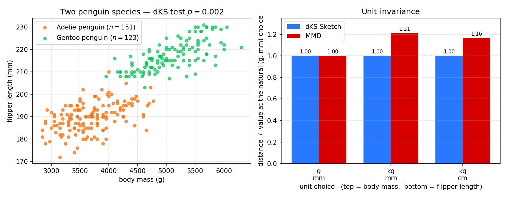
You can see it directly in the real-data examples below: switching body mass from grams to kilograms leaves dKS exactly unchanged, while a Gaussian-kernel MMD swings by 20–40%.
The idea
One number for how far apart two distributions are
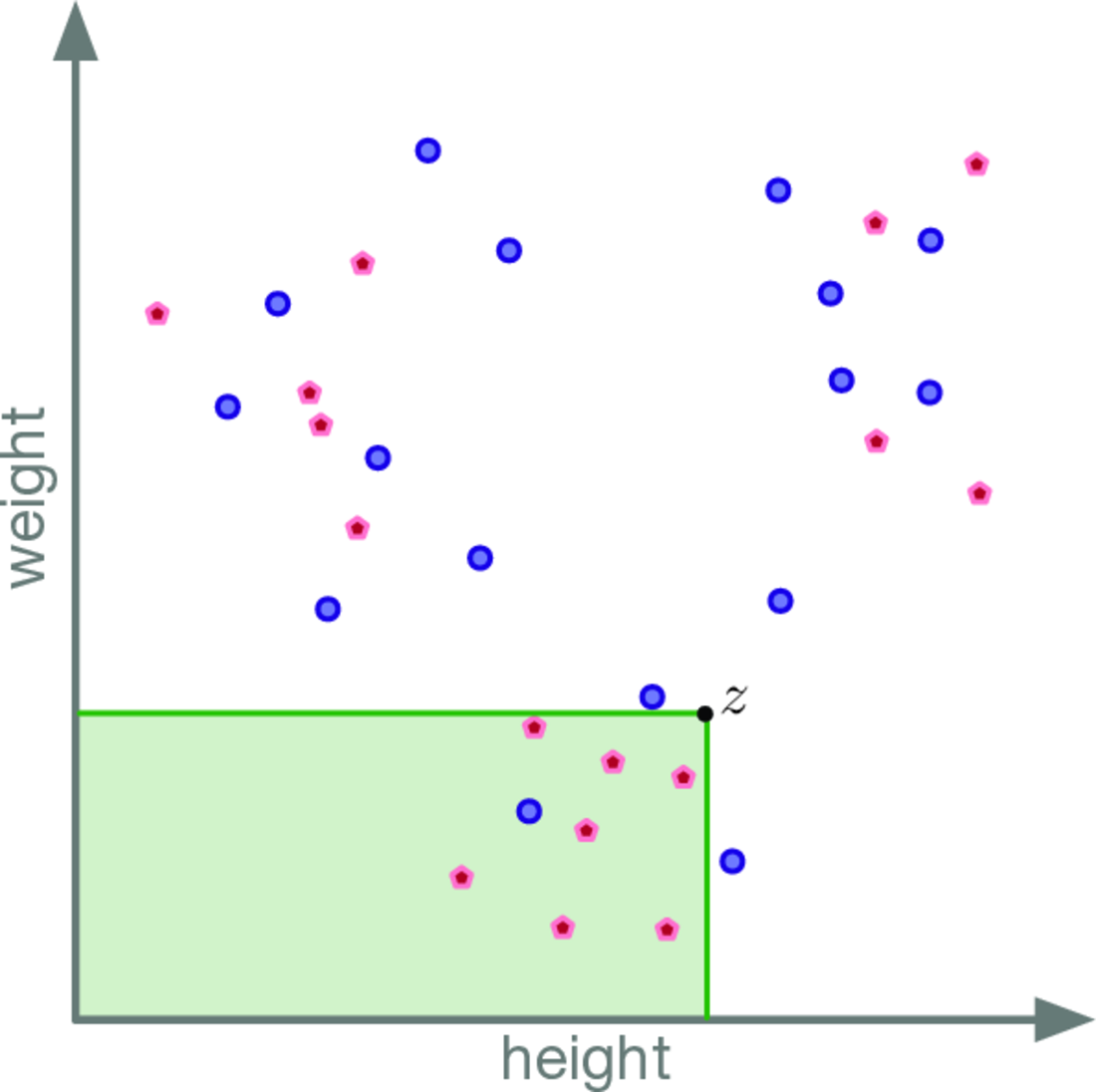
dKS is the largest gap between the two distributions' multivariate CDFs over lower-orthant ("dominating") rectangles. Because it uses coordinate order rather than Euclidean distance, it's invariant to each axis's units (height vs weight, temperature vs pressure), unlike MMD or Wasserstein.
Key contributions
What the paper establishes
A true metric
An integral probability metric with the strong identity property — a genuine metric on distributions, not just a pseudometric.
Light sample complexity
Only O((1/ε²)(d + log(1/δ))) samples to estimate — linear in the dimension, whatever the data's complexity.
Near-linear time
ε-approximable in O(n log n) for d = 2, and near-linear for d = 3, 4; going faster for d > 4 would break the Max-Weight-k-Clique conjecture.
A finite-sample test
A two-sample test with a guaranteed finite-sample bound on false positives — not asymptotic or Monte-Carlo.
Provably stable
One data point can swing the popular quad-KS variant, so it admits no sample-complexity bound; dKS does.
Results
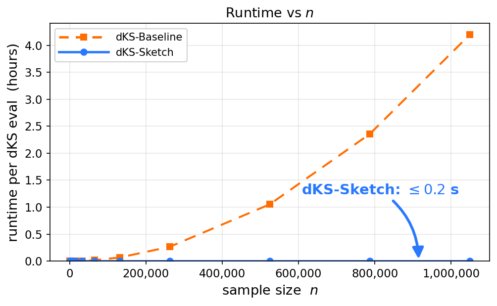
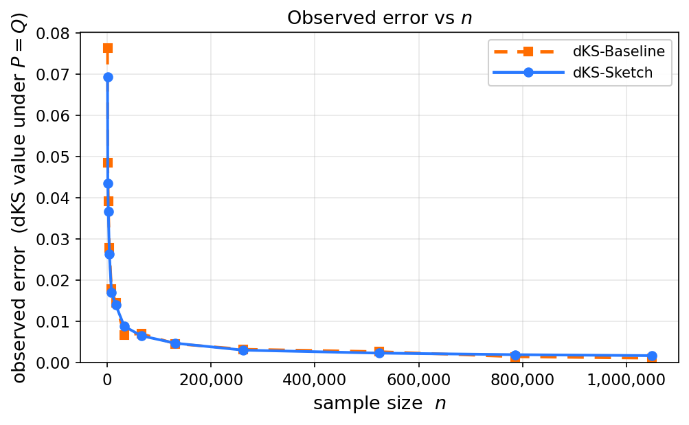
Fast to compute, accurate at the same rate
On real data
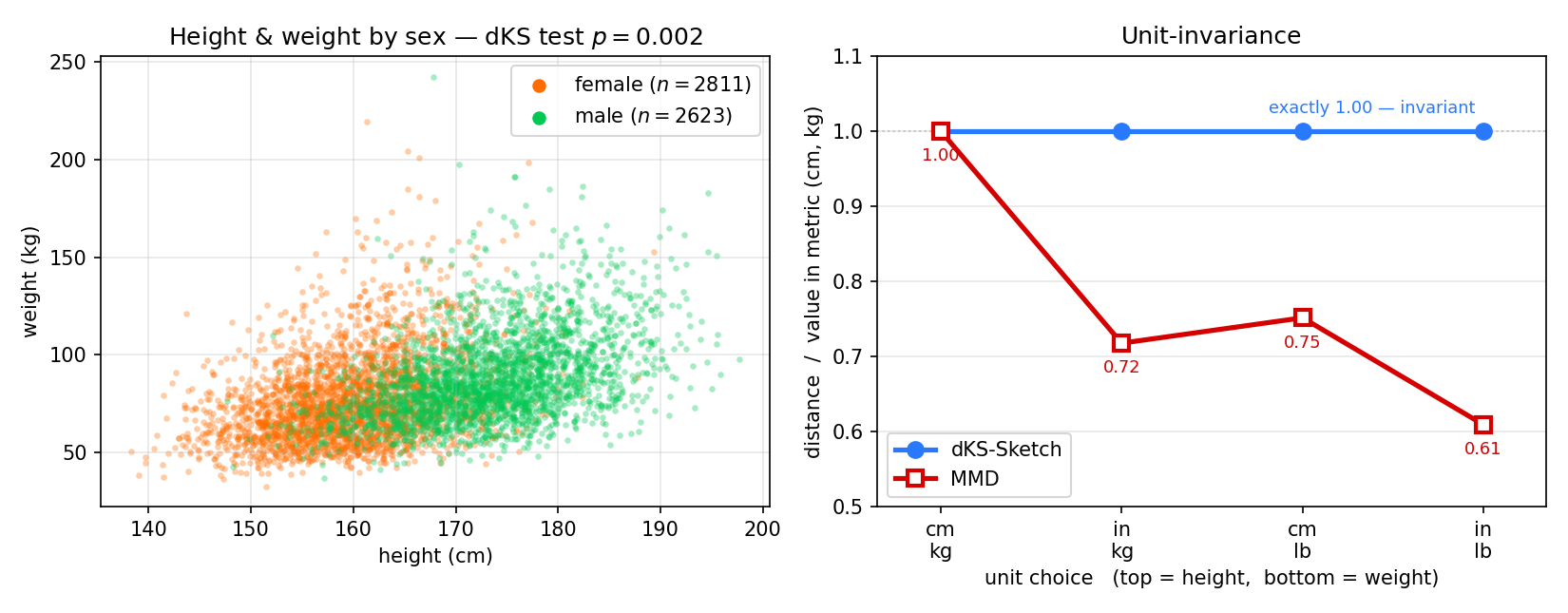
Unit-invariance, on two real datasets
Because dKS reads only the order of points along each axis, its answer doesn't change when an axis's units change. Here it is on two real datasets, beside a Gaussian-kernel MMD — which blends the axes through a Euclidean metric, so its answer depends on the units you happen to choose.
Palmer penguins — body mass vs flipper length
A dKS two-sample test cleanly separates Adelie from Gentoo penguins (p = 0.002). Switch body mass from grams to kilograms (with flipper length in mm or cm), and dKS-Sketch returns the identical value, while the Gaussian MMD shifts by up to 21%.
NHANES — height vs weight, metric vs US units
5,434 US adults from NHANES 2017–2018. The same person is “178 cm, 82 kg” in metric and “70 in, 181 lb” in US units. dKS-Sketch gives the identical answer for every metric/US choice; MMD changes by up to 39%.
Get started
A header-only library with Python bindings
C++
#include <dks/dks.hpp>
std::vector<dks::Point> P = {{0.1,0.2},{0.5,0.7}};
std::vector<dks::Point> Q = {{0.2,0.2},{0.6,0.8}};
double d = dks::approx(P, Q);   // fast,  O(n log n)
double e = dks::exact(P, Q);    // exact, O(n^2)
Python
import dks, numpy as np
P, Q = np.random.rand(1000,2), np.random.rand(1000,2)
print(dks.exact(P, Q), dks.approx(P, Q))
The full library, command-line tool, and reproducible experiments are available at the GitHub repository.
Citation
Cite this work
@article{jacobs2026dks,
  title   = {Efficient and Stable Multi-Dimensional Kolmogorov--Smirnov Distance},
  author  = {Jacobs, Peter Matthew and Namjoo, Foad and Phillips, Jeff M.},
  year    = {2026}
}